Line Models

In easyspec, we have a total of five line models available for fitting with the MCMC method.

All models are defined in terms of the line flux after continuum subtraction, \(F_{\lambda}\).

Gaussian Model

The Gaussian profile is defined by:

\[F_{\lambda} = A \exp\left(-\frac{(\lambda-\lambda_0)^2}{2\sigma^2}\right)\]

Parameters to fit:

• \(A\) - Amplitude

• \(\lambda_0\) - Mean wavelength (line center)

• \(\mathrm{FWHM}\) - Full width at half maximum, where \(\mathrm{FWHM} = 2\sigma\sqrt{2\ln 2}\)

Lorentzian Model

The Lorentzian profile is defined by:

\[F_{\lambda} = A \frac{\gamma^2}{(\lambda-\lambda_0)^2 + \gamma^2}\]

where \(\gamma = \mathrm{FWHM}/2\) is the half-width at half-maximum.

Parameters to fit:

• \(A\) - Amplitude

• \(\lambda_0\) - Mean wavelength (line center)

• \(\mathrm{FWHM}\) - Full width at half maximum, i.e., \(2\gamma\).

Note: The peak value occurs at \(\lambda = \lambda_0\) where \(F_{\lambda_0} = A\).

Voigt Model

The Voigt profile is a convolution of Gaussian and Lorentzian profiles, defined by:

\[F_{\lambda} = A \cdot V(\lambda; \lambda_0, \sigma, \gamma)\]

where the Voigt function \(V\) can be expressed as:

\[V(\lambda; \lambda_0, \sigma, \gamma) = \int_{-\infty}^{\infty} G(\lambda'; \sigma) L(\lambda - \lambda'; \gamma) d\lambda'\]

with \(G\) being the Gaussian and \(L\) the Lorentzian component.

Parameters to fit:

• \(A\) - Amplitude

• \(\lambda_0\) - Mean wavelength (line center)

• \(\mathrm{FWHM}_G\) - Gaussian \(\mathrm{FWHM} = 2\sigma\sqrt{2\ln 2}\)

• \(\mathrm{FWHM}_L\) - Lorentzian \(\mathrm{FWHM} =2\gamma\)

Skewed Gaussian Model

We start with the classical skewed Gaussian profile, defined by:

\[F_{\lambda} = A \exp\left(-\frac{(\lambda-\lambda_0)^2}{2\sigma^2}\right) \left[1 + \mathrm{erf}\left(\alpha\frac{\lambda-\lambda_0}{\sigma\sqrt{2}}\right)\right]\]

Where the parameters are:

• \(A\) - Amplitude

• \(\lambda_0\) - represents the center of the symmetric Gaussian component but does not correspond exactly to the peak position when skewness is significant.

• \(\sigma\) - Standard deviation

• \(\alpha\) - Skewness parameter

Note: When \(\alpha = 0\), the profile reduces to a standard Gaussian.

However, we rewrite this classical form of the skewed Gaussian in terms of \(\lambda_{\mathrm{peak}}\), i.e., the position of the line peak in the wavelength axis. We do that by solving for the relationship between the symmetrical-Gaussian line center \(\lambda_0\) and the actual peak position \(\lambda_{\mathrm{peak}}\).

The transformation is achieved through numerical root-finding. For a given skewness parameter \(s = \alpha/\sqrt{2}\) and dimensionless variable \(x = (\lambda_0-\lambda)/\sigma\), we solve the equation:

\[\frac{dF_{\lambda}}{dx} = -x [1 + \mathrm{erf}(s x)] + \frac{2s}{\sqrt{\pi}} e^{-s^2 x^2} = 0\]

using Brent’s method. The solution \(x_{\mathrm{peak}}\) gives us the offset between \(\lambda_0\) and \(\lambda_{\mathrm{peak}}\) through:

\[\lambda_0 = \lambda_{\mathrm{peak}} - x_{\mathrm{peak}} \sigma\]

The final implemented model uses the parameters:

• \(\lambda_{\mathrm{peak}}\) - Peak wavelength position (observed maximum)

• \(A\) - Amplitude of the Gaussian symmetrical component

• \(\mathrm{FWHM}_G\) - The \(\mathrm{FWHM} = 2\sigma\sqrt{2\ln 2}\) of the Gaussian symmetric component

• \(\alpha\) - Skewness parameter

This parameterization makes the fitting more physically intuitive, as \(\lambda_{\mathrm{peak}}\) directly corresponds to the observable line peak.

Skewed Lorentzian Model

We start with the classical skewed Lorentzian profile, defined by:

\[F_{\lambda} = A \frac{1 + \mathrm{erf}\left(\eta\frac{\lambda-\lambda_0}{\sqrt{2}\gamma}\right)}{1 + \frac{(\lambda-\lambda_0)^2}{\gamma^2}}\]

Where the parameters are:

• \(A\) - Amplitude

• \(\lambda_0\) - represents the center of the symmetric component but does not correspond exactly to the peak position when skewness is significant.

• \(\gamma\) - Lorentzian HWHM

• \(\eta\) - Skewness parameter

Note: When \(\eta = 0\), the profile reduces to a standard Lorentzian.

However, we rewrite this classical form of the skewed Lorentzian in terms of \(\lambda_{peak}\), i.e., the position of the line peak in the wavelength axis. We do that by solving for the relationship between the symmetrical-Lorentzian line center \(\lambda_0\) and the actual peak position \(\lambda_{\mathrm{peak}}\).

The transformation is achieved through numerical root-finding. If we define \(s = \eta/\sqrt{2}\) and \(x = \frac{\lambda-\lambda_0}{\gamma}\), the line peak occurs at \(\left.\frac{dF_{\lambda}}{dx}\right\vert_{x_{peak}} = 0\), which can be written as:

\[\frac{s}{\sqrt{\pi}} e^{-s^2 x^2} (1 + x^2) - x[1 + \mathrm{erf}(s x)] = 0\]

The solution \(x_{\mathrm{peak}}\) gives us the offset between \(\lambda_0\) and \(\lambda_{\mathrm{peak}}\) through:

\[\lambda_0 = \lambda_{\mathrm{peak}} - x_{\mathrm{peak}} \gamma\]

The final implemented model uses the parameters:

• \(\lambda_{\mathrm{peak}}\) - Peak wavelength position (observable maximum)

• \(A\) - Amplitude of the Lorentzian symmetrical component

• \(\mathrm{FWHM}_L\) - The \(\mathrm{FWHM} =2\gamma\) of the Lorentzian symmetric component

• \(\eta\) - Skewness parameter

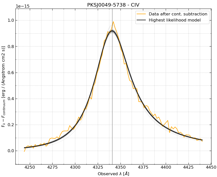
This parameterization makes the fitting more physically intuitive, as \(\lambda_{\mathrm{peak}}\) directly corresponds to the observable line peak. An example of a skewed Lorentzian profile applied to the CIV line of the AGN PKS J0049-5738 is shown below: